Articles in this Series
Preparatory Steps
Basic Classification (1/4) - Classifying Clothing on the MAC Mini M1
Basic Classification (2/4) - Tensorflow Lite Model Conversion
Basic Classification (3/4) - Machine Learning on TI's EdgeAI Cloud Tool (this article)
Interlude: TensorFlow Models on the Edge
Basic Classification (4/4) - EdgeAI Cloud - Jacinto ML Hardware Acceleration
Classification on the AI Edge
(5) SK-TDA4VM:Remote Login, Jupyter Notebook and Tensorflow.js
(6) SK-TDA4VM Starter Kit: Fashion Classification DNN
(7) Category List (link)
Introduction
In part 1 of this series, we trained a TensorFlow clothing classification model and then performed inferencing on several test items of clothing. Next, in the second article, we converted the model and exported it, as a TFLite file. Also, we tested the TFLite model in a TensorFlow interpreter. All the previous tasks have been completed on a Mac Mini M1, although any PC could have been used.
Now, the next stage in the workflow is to test our pre-trained clothing classification model on real hardware. Hence, in our quest to perform machine learning inferencing on the SK-TDA4VM Starter Kit, we move our pre-trained model to TI’s remote EdgeAI cloud server. That is, a Jacinto TDA4VM evaluation module hosted in a server room at Texas Instruments, otherwise known as the Cloud.
Hence, in this article we will perform inferencing on the Jacinto (TDA4VM processor), using the same code developed in the previous article. However, this time we will run it remotely in a Jupyter Notebook and to do so we will proceed, using the following steps:
- Log onto TI’s EdgeAI Cloud : https://dev.ti.com/edgeai/
- Save our TFLite model in our cloud workspace as ./mnist_tflite_models/model.tflite
- Download the Fashion MNIST test images set to our cloud workspace: ./samples/t10k-images-idx3-ubyte
- Download the Fashion MNIST test labels set to our cloud workspace: ./samples/t10k-labels-idx1-ubyte
- Launch a new Jupyter Notebook, configured to use a Tensorflow Lite runtime engine on a custom model, see Figure, below.
- Import our TFLite model, test images and labels
- Perform inferencing.
- Generate performance metrics.

Figure: The welcoming screen of TI’s EdgeAI Cloud. Click on the “Launch TI EDGE AI Cloud” label to access the remote Jupyter Notebook connected to the Jacinto Evaluation Module.
The TI EdgeAI Cloud is an easy-to-use software development environment provided by TI to evaluate embedded deep learning inference (free of charge). It provides a connection to a cloud hosted TDA4VM processor evaluation module .
Method Review and Analysis
Up until now we have developed a python inferencing runtime module without looking into the details of how it actually works. Therefore, as the code has not changed that much, now is a good time to dive under the hood to investigate
- How to setup the TFLite interpreter runtime
- Use it to perform inferencing
- Use it to predict results.
A summary of the basic deep learning model, trained to classify clothing, is shown immediately, below. It consists of a single input layer, a fully connected inner layer and an output layer.
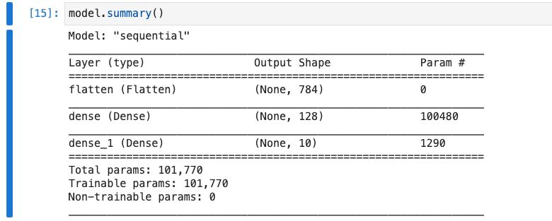
Figure: Fashion Classification Model Summary. Input layer (flatten), Inner layer (dense), Output layer (dense_1)
A snippet of the lines of code of interest, taken from the Jupyter Notebook Section below, is shown, next:
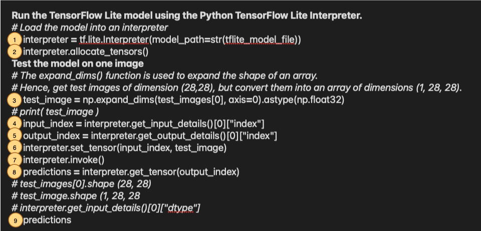
Lets dissect each line one at at time.
- interpreter = tf.lite.Interpreter(model_path=str(tflite_model_file))
Initially, we setup the interpreter to only load our TFLite model, although the interpreter can be initialised with many more parameters. The full interpreter function interface is shown, below.
tf.lite.Interpreter (
model_path=None,
model_content=None,
experimental_delegates=None,
num_threads=None,
experimental_op_resolver_type=tf.lite.experimental.OpResolverType.AUTO,
experimental_preserve_all_tensors=False
)
One of the more interesting input parameters is the experimental_delegates. We will set this parameter, in the next article, to implement inferencing on the Jacinto evaluation module’s hardware accelerator. For now we will leave it uninitialised to use the dual ARM A72 CPUs.
- interpreter.allocate_tensors()
This function initialises the deep learning graph with the weight and node values read from the imported TFLite model.
N.B tensors are multi-dimensional arrays with a uniform type (called a dtype). They are similar to NumPy, where tensors are (kind of) like np.arrays. All tensors are immutable like Python numbers and strings: you can never update the contents of a tensor, only create a new one.
- test_image = np.expand_dims(test_images[0], axis=0).astype(np.float32)
Here, we are extracting the first test image and expanding it from a 2-dimensional (28,28) array to a batch size, 3-dimensional (1,28,28) array. The test image is supplied, as the input data to the deep neural network (see item 6, below).
- input_index = interpreter.get_input_details()[0]["index"]
The get_input_details() returns the details of the model’s input tensor. That is the flatten layer (see model summary, above).
- output_index = interpreter.get_output_details()[0]["index"]
The get_output_detials() returns the details of the model’s output tensor. That is the dense_1 layer (See model summary, above.)
- interpreter.set_tensor(input_index, test_image)
The set_tensor() initialises the value of the input tensor to the test image (1,28,28) array we preformatted earlier, in item 3 above. Note this copies the test image data by value. Other functions exists to pass the input data by reference.
- interpreter.invoke()
This function invokes the interpreter to perform inferencing on the test image set previously. According to the TensorFlow documentation “Be sure to set the input sizes, allocate tensors and fill values before calling this. Also, note that this function releases the GIL so heavy computation can be done in the background while the Python interpreter continues. No other function on this object should be called while the invoke() call has not finished” .
- predictions = interpreter.get_tensor(output_index)
Gets a copy of the value of the output tensor. The function returns the model's linear outputs, logits. Attach a softmax layer to convert the logits to probabilities, which are easier to interpret. If you wish to avoid the copy, use tensor(). This function cannot be used to read intermediate results. A, typical, output from this function is given, below, where the largest value corresponds to the predicted output.
array([[ -6.9800515 , -17.512352, -7.672169, -15.466933, -10.164105, -0.97598296, -9.541937, 2.114148, -8.446375 , 6.7880406 ]], dtype=float32)
In this case an ankle boot (Item 9) has been predicted.
Conclusion
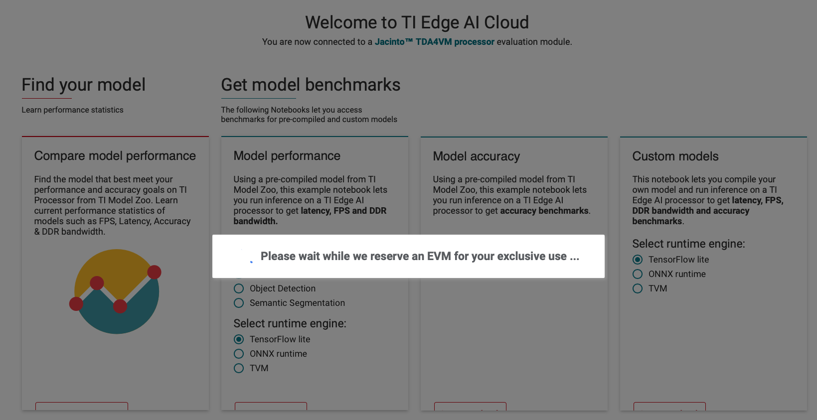
Figure: When you logon to the TI Edge AI Cloud you are allocated a Jacinto EVM for your exclusive use for 3 hours. Hence, it's imperative to save your work regularly, as when your 3 hours are up you will be booted off the server!
So what have we achieved in this article? We are now one step away from performing inferencing on the SK-TDA4VM’s hardware accelerators. Presently, we are able to run our clothing classification model on TI’s EdgeAI cloud server, all be it, using the dual ARM A72 processors. In the next article we will perform the same exercise, but this time we will make a slight adjustment, to our Jupyter Notebook, to use the TIDL delegate that triggers Deep Learning hardware acceleration. The Jupyter Notebook used for this article is listed below.
References
- Fashion MNIST Dataset
- stackoverflow: How to import pre-downloaded MNIST dataset from a specific directory or folder?
- Why does "pip install" inside Python raise a SyntaxError?
Jupyter Notebook
Setup the environment
import os
import tqdm
import cv2
import numpy as np
import tflite_runtime.interpreter as tflite
import matplotlib.pyplot as plt
import pathlib
We need to download the test images and labels from Github https://github.com/zalandoresearch/fashion-mnist
t10k-images-idx3-ubyte - test set images
t10k-labels-idx1-ubyte - test set labels
Save them to a 'My Workspace' folder e.g samples/.
To load the images we require mnist. Hence, get the python-mnist package from PyPi: Alternatively, we could load the images directly into a numpy array using the id2xnumpy package
#pip install idx2numpy
#import idx2numpy
#import numpy as np
#file = 'samples/t10k-images-idx3-ubyte'
#arr = idx2numpy.convert_from_file(file)
#arr is now a np.ndarray type of object of shape (10000, 28, 28)
# Lets do the former.
import pip

#package_names=['selenium', 'requests'] #packages to install
package_names=['python-mnist'] #packages to install
pip.main(['install'] + package_names + ['--upgrade'])
# --upgrade to install or update existing packages
Requirement already up-to-date: python-mnist in /usr/local/lib/python3.6/dist-packages
0
from mnist import MNIST

mndata = MNIST('samples')

# Each image of the test_images list is a Python list of unsigned bytes.
# The labels are a Python array of unsigned bytes, too.
test_images, test_labels = mndata.load_testing()

# Confirm that we have loaded the 10k test images ...
len(test_images)

# However the test images have been imported as a (10000, 784) list so we need to
#  convert them into (10000, 28, 28) of type ?
# Each image can be converted, using the following line of code.
# Where index is the array index number
# image = np.reshape(test_images[index], (28, 28))
10000
# Confirm that we have 10k labels.
len(test_labels)
10000
The labels are an array of integers, ranging from 0 to 9. These correspond to the class of clothing the image represents:
| Label | Class |
|---|---|
| 0 | T-shirt/top |
| 1 | Trouser |
| 2 | Pullover |
| 3 | Dress |
| 4 | Coat |
| 5 | Sandal |
| 6 | Shirt |
| 7 | Sneaker |
| 8 | Bag |
| 9 | Ankle boot |
Each image is mapped to a single label. Since the class names are not included with the dataset, store them here to use later when plotting the images:
class_names = ['T-shirt/top', 'Trouser', 'Pullover', 'Dress', 'Coat',
               'Sandal', 'Shirt', 'Sneaker', 'Bag', 'Ankle boot']

class_names[ test_labels[1] ]
'Pullover'
index = 100
# Images are loaded as 1D (1,784) arrays. Hence, convert them to 2D (28,28)
image = np.reshape(test_images[index], (28, 28))
plt.figure()
plt.imshow(image)
plt.colorbar()
plt.grid(False)
plt.xlabel(class_names[test_labels[index]])
plt.show()

tflite_models_dir = pathlib.Path("./mnist_tflite_models/")
tflite_model_file = pathlib.Path(tflite_models_dir/'model.tflite')

interpreter = tflite.Interpreter(model_path=str(tflite_model_file))
interpreter.allocate_tensors()
test_image = np.expand_dims(image, axis=0).astype(np.float32)
input_index = interpreter.get_input_details()[0]["index"]
output_index = interpreter.get_output_details()[0]["index"]
interpreter.set_tensor(input_index, test_image)
interpreter.invoke()
predictions = interpreter.get_tensor(output_index)
predictions
array([[ -282.43134, -1012.56415,  -790.8751 ,  1327.3641 , -1204.9701 ,
        -2262.4978 ,  -455.5687 , -3505.6287 , -1154.8307 , -2359.497  ]],
      dtype=float32)
Additional Material
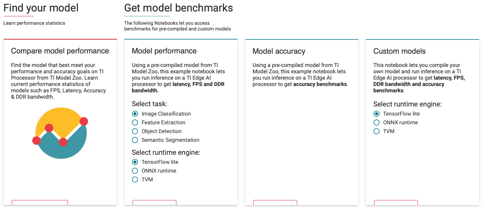
Figure: When you launch the TI Edge AI Cloud Server a Jacinto EVM is reserved for your exclusive use. That is, you are allotted an EVM to use for the next three hours. For our task, since we are using our custom TFLite fashion classification model, we choose the Tensorflow Lite option.
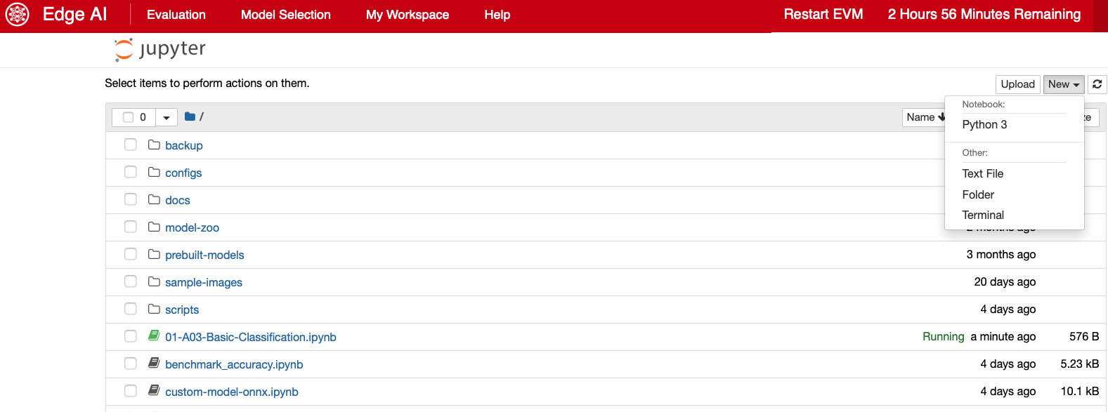
Figure: Launch a Python 3 notebook. N.B There doesn't appear to be a console option.
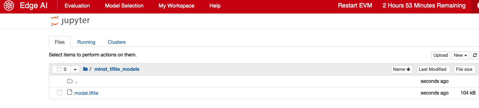
Figure: Upload the model.tflite file, we created in the previous article, to your workspace. In my case I saved the model in the ./mnist_tflite_models directory.
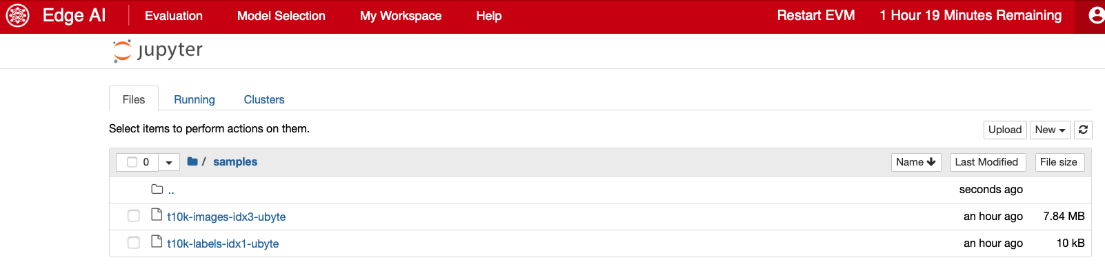
Figure: For this exercise I have also uploaded the Fashion MNIST test images and labels to the ./samples folder.