: Written by: BP; Category: Edge AI: Machine Learning Classification; Published: 03 November 2021

Articles in this Series

Preparatory Steps

Basic Classification (1/4) - Classifying Clothing on the Mac Mini M1 (this article)

Basic Classification (2/4) - Tensorflow Lite Model Conversion

Basic Classification (3/4) - Machine Learning on TI's EdgeAI Cloud

Interlude: TensorFlow Models on the Edge

Basic Classification (4/4) - EdgeAI Cloud - Jacinto ML Hardware Acceleration

Classification on the AI Edge

(5) SK-TDA4VM:Remote Login, Jupyter Notebook and Tensorflow.js

(6) SK-TDA4VM Starter Kit: Fashion Classification DNN

(7) - Category List

Introduction

This is the first article, as part of a series of four, developed to better understand TI’s recommended workflow for running machine learning inferencing algorithms on the SK-TDA4VM starter kit. The motivation for running this series has been discussed in the previous blog post SK-TDA4VM - On the Artificial Intelligence Edge. In this article I’ll be running the Tensorflow Fashion MNIST beginners tutorial on the Mac Mini M1, although any personal computer will do.

The first step in running the Fashion MNIST classification on the Mac M1 is to install Tensorflow and the Tensorflow metal plugin. The plugin accelerates inferencing, by using the M1’s neural engine, which performs ML inferencing up to x15 faster on the GPU, compared to the 8-core CPU.

There are many Mac M1 tutorials online that describe how to install Tensorflow and Jupiter labs in a python virtual environment. The more up to date installation methods take advantage of the Tensorflow delegate architecture, which leverages the M1’s GPU. Due to the continued evolution of Miniforge and Tensorflow on the Mac M1 I will only list the installation steps I followed here, a more up to date method should be found by Googling.

These are the steps I followed to enable machine learning on the Apple Silicon Mac M1, natively. The installation supports TensorFlow 2.6 GPU acceleration (tensorflow-metal PluggableDevice):

Install Miniforge for OSX, using the arm 64 (Apple Silicon) architecture - miniforge3-MacOSX-arm64
Create and activate a python (3.9.5) virtual environment.
Install Tensorflow dependencies
Install Tensorflow-macos
Install Tensorflow-metal
Install needed packages

libjpeg
Matplotlib
jupyterlab

That’s it, at this point I was good to go . Although to actually get Tensorflow to run successfully I needed to upgrade MacOS to Monterey 12.0. Also, I installed the GNU Octave notebook extension for some upcoming DSP projects.

The Fashion-MNIST dataset

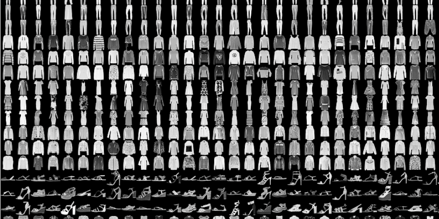
Fashion-MNIST is a dataset of Zelando’s article images consisting of a training set of 60,000 examples and a test set of 10,000 examples. Each example is a 28x28 grayscale image, associated with a label from 10 classes. We intend Fashion-MNIST to serve as a direct drop-in replacement for the original MNIST dataset for benchmarking machine learning algorithms. It shares the same image size and structure of training and testing splits. - Reference: Fashion-NIST (https://github.com/zalandoresearch/fashion-mnist)

Jupiter Notebook Fashion-MNIST Classification

Fashion-MNIST is a dataset consisting of a training set of 60,000 examples and a test set of 10,000 examples. Each example is a 28x28 pixel grayscale image, associated with a label from 10 classes.

In [118]:

# TensorFlow and tf.keras
import tensorflow as tf

# Helper libraries
import numpy as np
import matplotlib.pyplot as plt
from os import getcwd

print('\u2022 Using TensorFlow Version:', tf.__version__)
print('\u2022 GPU Device Found.' if tf.test.is_gpu_available() else '\u2022 GPU Device Not Found. Running on CPU')

• Using TensorFlow Version: 2.6.0
• GPU Device Found.

2021-10-31 14:59:28.709594: I tensorflow/core/common_runtime/pluggable_device/pluggable_device_factory.cc:305] Could not identify NUMA node of platform GPU ID 0, defaulting to 0. Your kernel may not have been built with NUMA support.
2021-10-31 14:59:28.711011: I tensorflow/core/common_runtime/pluggable_device/pluggable_device_factory.cc:271] Created TensorFlow device (/device:GPU:0 with 0 MB memory) -> physical PluggableDevice (device: 0, name: METAL, pci bus id: <undefined>)

Import the Fashion MNIST training and test datasets into four NumPy arrays. Each image is 28 x 28 pixels.

In [119]:

fashion_mnist = tf.keras.datasets.fashion_mnist

(train_images, train_labels), (test_images, test_labels) = fashion_mnist.load_data()

The images are 28x28 NumPy arrays, with pixel values ranging from 0 to 255. The labels are an array of integers, ranging from 0 to 9. These correspond to the class of clothing the image represents:

Label	Class
0	T-shirt/top
1	Trouser
2	Pullover
3	Dress
4	Coat
5	Sandal
6	Shirt
7	Sneaker
8	Bag
9	Ankle boot

Each image is mapped to a single label. Since the class names are not included with the dataset, store them here to use later when plotting the images:

In [120]:

class_names = ['T-shirt/top', 'Trouser', 'Pullover', 'Dress', 'Coat',
               'Sandal', 'Shirt', 'Sneaker', 'Bag', 'Ankle boot']

In [121]:

train_images.shape

Out[121]:

(60000, 28, 28)

In [122]:

len(train_labels)

Out[122]:

In [123]:

train_labels

Out[123]:

array([9, 0, 0, ..., 3, 0, 5], dtype=uint8)

In [124]:

len(test_labels)

Out[124]:

In [125]:

test_images.shape

Out[125]:

(10000, 28, 28)

In [126]:

plt.figure()
plt.imshow(train_images[1])
plt.colorbar()
plt.grid(False)
plt.show()

The images have greyscale values, between 0 and 255. Hence scale the values, between 0 and 1.

In [127]:

train_images = train_images / 255.0

test_images = test_images / 255.0

Display a couple of images.

In [128]:

plt.figure(figsize=(10,10))
for i in range(25):
    plt.subplot(5,5,i+1)
    plt.xticks([])
    plt.yticks([])
    plt.grid(False)
    plt.imshow(train_images[i], cmap=plt.cm.binary)
    plt.xlabel(class_names[train_labels[i]])
plt.show()

Build the Model

The first layer in this network, tf.keras.layers.Flatten, transforms the format of the images from a two-dimensional array (of 28 by 28 pixels) to a one-dimensional array (of 28 * 28 = 784 pixels). After the pixels are flattened, the network consists of a sequence of two tf.keras.layers.Dense layers. These are densely connected, or fully connected, neural layers. The first Dense layer has 128 nodes (or neurons). The second (and last) layer returns a logits array with length of 10. Each node contains a score that indicates the current image belongs to one of the 10 classes.

In [129]:

model = tf.keras.Sequential([
    tf.keras.layers.Flatten(input_shape=(28, 28)),
    tf.keras.layers.Dense(128, activation='relu'),
    tf.keras.layers.Dense(10)
])

Compile the model

Before the model is ready for training, it needs a few more settings. These are added during the model's compile step:

Loss function —This measures how accurate the model is during training. You want to minimize this function to "steer" the model in the right direction. Optimizer — This is how the model is updated based on the data it sees and its loss function. Metrics — Used to monitor the training and testing steps. The following example uses accuracy, the fraction of the images that are correctly classified.

In [130]:

model.compile(optimizer='adam',
              loss=tf.keras.losses.SparseCategoricalCrossentropy(from_logits=True),
              metrics=['accuracy'])

Train the Model

To start training, call the model.fit method—so called because it "fits" the model to the training data:

In [131]:

model.fit(train_images, train_labels, epochs=10)

Epoch 1/10
  35/1875 [..............................] - ETA: 5s - loss: 1.3832 - accuracy: 0.5491

2021-10-31 14:59:30.405955: I tensorflow/core/grappler/optimizers/custom_graph_optimizer_registry.cc:112] Plugin optimizer for device_type GPU is enabled.

1875/1875 [==============================] - 6s 3ms/step - loss: 0.5015 - accuracy: 0.8231
Epoch 2/10
1875/1875 [==============================] - 5s 3ms/step - loss: 0.3748 - accuracy: 0.8649
Epoch 3/10
1875/1875 [==============================] - 5s 3ms/step - loss: 0.3356 - accuracy: 0.8772
Epoch 4/10
1875/1875 [==============================] - 5s 3ms/step - loss: 0.3115 - accuracy: 0.8838
Epoch 5/10
1875/1875 [==============================] - 5s 3ms/step - loss: 0.2916 - accuracy: 0.8931
Epoch 6/10
1875/1875 [==============================] - 5s 3ms/step - loss: 0.2789 - accuracy: 0.8951
Epoch 7/10
1875/1875 [==============================] - 5s 3ms/step - loss: 0.2649 - accuracy: 0.9004
Epoch 8/10
1875/1875 [==============================] - 5s 3ms/step - loss: 0.2524 - accuracy: 0.9061
Epoch 9/10
1875/1875 [==============================] - 5s 3ms/step - loss: 0.2446 - accuracy: 0.9092
Epoch 10/10
1875/1875 [==============================] - 5s 3ms/step - loss: 0.2372 - accuracy: 0.9108

Out[131]:

<keras.callbacks.History at 0x156534bb0>

Evaluate the model accuracy

Next, compare how the model performs on the test dataset:

In [132]:

test_loss, test_acc = model.evaluate(test_images,  test_labels, verbose=2)

print('\nTest accuracy:', test_acc)

2021-10-31 15:00:24.988052: I tensorflow/core/grappler/optimizers/custom_graph_optimizer_registry.cc:112] Plugin optimizer for device_type GPU is enabled.

313/313 - 1s - loss: 0.3345 - accuracy: 0.8804

Test accuracy: 0.8804000616073608

Make predictions

With the model trained, you can use it to make predictions about some images. The model's linear outputs, logits. Attach a softmax layer to convert the logits to probabilities, which are easier to interpret.

In [133]:

probability_model = tf.keras.Sequential([model, 
                                         tf.keras.layers.Softmax()])

In [134]:

predictions = probability_model.predict(test_images)

2021-10-31 15:00:25.763975: I tensorflow/core/grappler/optimizers/custom_graph_optimizer_registry.cc:112] Plugin optimizer for device_type GPU is enabled.

In [135]:

predictions[0]

Out[135]:

array([3.3962785e-08, 5.2536460e-12, 4.5928550e-10, 1.3885787e-11,
       7.6916924e-11, 2.2161782e-02, 6.3888947e-08, 3.9380090e-03,
       3.7821670e-09, 9.7390002e-01], dtype=float32)

Graph the predictions to look at the full set of 10 class predictions.

In [136]:

def plot_image(i, predictions_array, true_label, img):
  true_label, img = true_label[i], img[i]
  plt.grid(False)
  plt.xticks([])
  plt.yticks([])

  plt.imshow(img, cmap=plt.cm.binary)

  predicted_label = np.argmax(predictions_array)
  if predicted_label == true_label:
    color = 'blue'
  else:
    color = 'red'

  plt.xlabel("{} {:2.0f}% ({})".format(class_names[predicted_label],
                                100*np.max(predictions_array),
                                class_names[true_label]),
                                color=color)

def plot_value_array(i, predictions_array, true_label):
  true_label = true_label[i]
  plt.grid(False)
  plt.xticks(range(10))
  plt.yticks([])
  thisplot = plt.bar(range(10), predictions_array, color="#777777")
  plt.ylim([0, 1])
  predicted_label = np.argmax(predictions_array)

  thisplot[predicted_label].set_color('red')
  thisplot[true_label].set_color('blue')

In [137]:

i = 0
plt.figure(figsize=(6,3))
plt.subplot(1,2,1)
plot_image(i, predictions[i], test_labels, test_images)
plt.subplot(1,2,2)
plot_value_array(i, predictions[i],  test_labels)
plt.show()

In [138]:

i = 12
plt.figure(figsize=(6,3))
plt.subplot(1,2,1)
plot_image(i, predictions[i], test_labels, test_images)
plt.subplot(1,2,2)
plot_value_array(i, predictions[i],  test_labels)
plt.show()

In [139]:

# Plot the first X test images, their predicted labels, and the true labels.
# Color correct predictions in blue and incorrect predictions in red.
num_rows = 5
num_cols = 3
num_images = num_rows*num_cols
plt.figure(figsize=(2*2*num_cols, 2*num_rows))
for i in range(num_images):
  plt.subplot(num_rows, 2*num_cols, 2*i+1)
  plot_image(i, predictions[i], test_labels, test_images)
  plt.subplot(num_rows, 2*num_cols, 2*i+2)
  plot_value_array(i, predictions[i], test_labels)
plt.tight_layout()
plt.show()

In [140]:

# Grab an image from the test dataset.
img = test_images[1]

print(img.shape)

(28, 28)

In [141]:

# Add the image to a batch where it's the only member.
img = (np.expand_dims(img,0))

print(img.shape)

(1, 28, 28)

In [142]:

predictions_single = probability_model.predict(img)

print(predictions_single)

[[4.2759009e-05 8.0097751e-12 9.9578261e-01 3.2288022e-10 3.3681127e-03
  3.4885767e-14 8.0647180e-04 3.3935744e-18 7.4961015e-10 1.2566573e-13]]

In [143]:

plot_value_array(1, predictions_single[0], test_labels)
_ = plt.xticks(range(10), class_names, rotation=45)
plt.show()

In [144]:

np.argmax(predictions_single[0])

Out[144]:

Conclusion

In this article I have trained and used the Fashion-MNIST dataset to infer items of clothing on the Mac Mini M1, using the M1's GPU (Can we use the neural compute engine?). Hence, the first stage of running machine learning inferencing models on the SK-TDA4VM starter kit has been completed. However, it should be noted that this first stage could have been implemented on any PC. The next stage requires converting the model created in this stage into a TensorFlow Lite model, which will be the topic of discussion in the next article in this series.

Machine Learning Basic Classification (1/4): On the Mac Mini M1